Fractal geometry is used for measuring “complexity” in a variety of ways (Mitchell, 1996). Fractal measures can
identify non-linear relationships in data and scale invariant behaviors. Fractal dimension has been used for feature
selection when analyzing data sets (Traina, 2000). Fractal dimension has also been shown to be effective in
recognizing diabetic patients from retinal images (Cheng, 2003). Kotowski et al. has conjectured that entropy
measures and specifically fractal dimension can be used to characterize classes of genetic algorithms and their
properties in terms of convergence. Fractal dimension has been used to model the trajectory of genetic algorithms
and is proposed as a new method for constructing GAs and optimizing them (Kotowski, 2008).
Fractal dimension (FD) offers a measure for assessing the self-similarity of a branching pattern such as those
discussed above. Self- similar patterns will generally have higher fractal dimension. This is because self-similar
patterns have detail at many levels and fill the 2 dimensional plane more than a Euclidean object with comparable
detail at a given level. In general, a self-similar fractal object obeys the following relation:
N = Md
Where d is the fractal dimension (or fractional dimension) and M is the number of segments in the initial object,
called the initiator, and N is the resulting number of elements produced, called the generator. Fractals typically have
fractional dimensions; that is, dimensions that lie between whole integer values. A fractal (fractional) dimension is more like a measure of density or a rate of growth towards infinity than a conventional description of space. The
exponent d is the Hausdorff dimension. You can solve this equation for d by taking the logarithm of both sides and
re-arranging:
d = log N / log M
What this tells us is that the dimension of a fractal increases as the number of copies increases, and decreases as the
scaling fraction decreases. (Note that d will be the same no matter what the base of the logarithm as long as the logs
in the numerator and denominator have the same base.) This measure of dimension can be applied to objects that we
are familiar with, such as lines, squares, and cubes, where the result is exactly as expected.
Box-counting dimension is often used to measure fractals that are not defined with pure geometry but rather consists
of idiosyncratic shapes such as those found in nature and in complex, hard-to-characterize forms such as cities. Boxcounting
dimension is determined by first overlaying a grid on an image and counting how many lattice sites or
‘boxes’ are necessary to completely cover the shape. Additional grids at ever decreasing or increasing scales are
overlaid recursively on the shape. The coordinates of the log of number of boxes Nε and the of log of their scaling
ration, 1/ε are recorded in a scatter plot. The scatter plot is a graph with log 1/ε along the x-axis and log Nε along the
y-axis. From the scatter plot a best-fit line or sum of least squares linear regression is drawn. The slope of the best fit
line is the fractal dimension of the shape and should approximate the Hausdorff dimension.
Box-counting dimension uses the same idea as fractal dimension but applied generally to any number of scaled
‘boxes’ superimposed on an object:
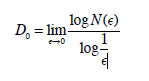
Where D is the box‐counting dimension and N is the number of boxes covering an object and ε is the scaling ratio.